GitHub: Code Samples / Volumetric-Fog
Specialization
As part of The Game Assembly’s specialization course, we were given the opportunity to choose an area of focus and develop a larger technical feature over ~3–4 weeks (half-time).
I chose to implement volumetric fog — mainly because of how impactful it is visually. Fog adds depth, atmosphere, and mood to a scene in a way that’s immediately noticeable, even to non-technical players. It helps ground lighting and makes scenes feel more cohesive. A few simple controls — global density, height, and local volumes — are enough to get compelling results quickly, while still being grounded in physically-based light transport. Clustered Lighting was also implemented in addition to better support and optimize the volumetric fog.
My implementation is largely inspired by the approach presented by Sébastien Hillaire at Frostbite — Physically-Based Unified Volumetric Rendering in Frostbite. PBRT was the other key resource, particularly for building intuition around the underlying theory.
Special Thanks
- Alex Tardif — for serving as my mentor throughout this project. His feedback, insights, and availability made a real difference in both the implementation and my understanding of the problem.
- Sébastien Hillaire — for the original froxel-based volumetric fog presentation this work is heavily inspired by, and for taking the time to answer questions and clarify key parts of the technique.
Theory
Before diving into the implementation, it helps to understand what’s actually happening when light moves through fog or smoke. This section won’t go deep into the full physics — it’s meant as an approachable overview you can reference as you read through the rest of the post. If you want to go deeper, PBRT covers volume scattering processes thoroughly in Chapter 11 and volume light transport in Chapter 15.
The Core Idea
When light travels through a participating medium (fog, smoke, dust), two things happen simultaneously:
- Light is attenuated — some of it is absorbed or scattered away before reaching the camera
- Light is added — particles in the medium redirect incoming light toward the camera
So the color you see at any pixel is a mix of two things: light from surfaces behind the fog, dimmed by it, and light contributed by the fog itself.
Transmittance — How Fog Dims the World
Transmittance is what causes distant objects to fade into fog.
Transmittance describes how much light survives as it passes through the medium:
$$ T_r \approx e^{-\sigma_t \cdot d} $$
- \(\sigma_t\) is the extinction coefficient — how dense or opaque the medium is
- \(d\) is the distance traveled through it
The intuition is simple: the denser the fog, or the further light has to travel through it, the less of it reaches the camera. This is what causes distant objects to fade out.
Scattering — How Fog Glows
Scattering is what makes fog visible in the first place. Rather than only receiving light from surfaces, each point in the volume also picks up light from surrounding sources and redirects some of it toward the camera.
For each light source, we evaluate:
$$L_{scat} = \rho \sum_{lights} f(v, l)\ Vis(x, l)\ L_i(x, l)$$
In plain terms: take the light’s intensity, check if the point is in shadow, apply the phase function to determine how much scatters toward the camera, then scale by the medium’s albedo. Sum that up for all lights.
The phase function \(f(v, l)\) is worth calling out specifically — it controls the shape of scattering:
- Strong forward scattering produces visible light shafts and god rays
- Uniform scattering produces softer, more diffuse fog
Putting It Together
The full volumetric rendering equation combines both effects:
$$L_i = T_r \cdot L_{surface} + \int_0^s T_r(x, x_t)\ \sigma_t(x)\ L_{scat}(x_t)\ dt$$
The first term is attenuated surface light. The second accumulates in-scattered light along the view ray. Evaluating that integral in real-time is the core challenge — which is what the froxel-based approach in the implementation section is all about.
Quick Glossary
| Term | Symbol | Meaning |
|---|---|---|
| Absorption | \(\sigma_a\) | Light absorbed and lost entirely |
| Scattering | \(\sigma_s\) | Light redirected toward the camera |
| Extinction | \(\sigma_t\) | Total loss: \(\sigma_a + \sigma_s\) |
| Albedo | \(\rho\) | Ratio of scattered to total extinction: \(\sigma_s / \sigma_t\) |
| Transmittance | \(T_r\) | Fraction of light that survives: \(e^{-\sigma_t \cdot d}\) |
| Phase function | \(f(v, l)\) | Directional distribution of scattering |
| In-scattered light | \(L_{scat}\) | Light added to the view by the medium |
Real-Time Integration
Evaluating the scattering integral continuously along the ray is expensive. The trick is to assume that scattering and extinction are constant within each froxel, which lets the integral be solved analytically:
$$\int_0^D e^{-\sigma_t x} \cdot S\ dx = \frac{S - S \cdot e^{-\sigma_t D}}{\sigma_t}$$
This closed-form solution is what makes stable, efficient froxel integration possible — and it’s the foundation of everything in the implementation that follows.
Implementation
The implementation breaks down into three compute passes that map directly onto the theory:
- Voxelization — fill the froxel grid with media properties
- Lighting — evaluate light contribution at every froxel
- Ray Marching — integrate front-to-back and composite into the scene
Each pass builds on the previous one, and together they approximate the full volumetric rendering equation from the theory section. But before any of that, we need a structure to work in.
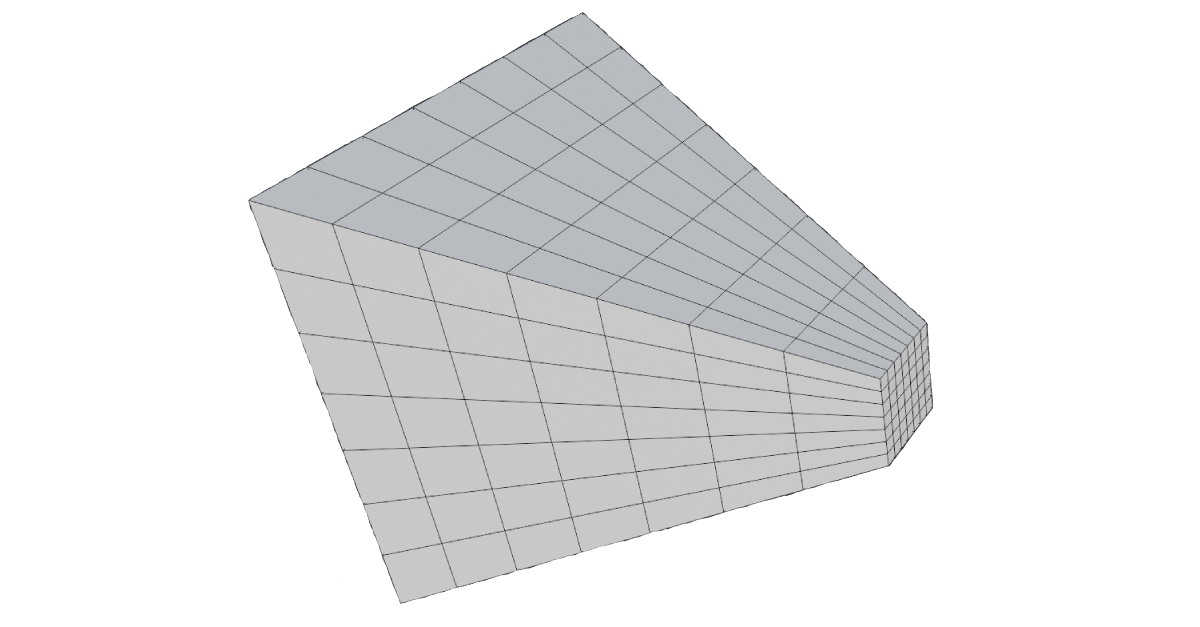
Froxels
A froxel (frustum voxel) is the volumetric equivalent of a pixel. Where a pixel represents a point on the screen, a froxel represents a small chunk of the camera frustum in 3D space. Together, they form a 3D grid that covers everything the camera can see — the froxel grid.
The XY dimensions of the grid map directly to screen space. Rather than allocating one froxel per pixel, the screen is divided into tiles:
static constexpr uint32_t TILE_SIZE{ 8 }; // froxel XY downscale
So a 1920×1080 screen becomes a 240×135 grid in XY. The Z dimension represents depth slices into the frustum:
static constexpr uint32_t FROXEL_Z{ 64 }; // depth slices
This gives a final grid of 240×135×64 froxels — each one a small frustum-shaped cell storing the fog properties for that region of space.
Depth Distribution
How you slice depth is not obvious. A uniform distribution — splitting the view range into equal intervals — wastes most of your slices on distant regions where detail is less important, while leaving the area near the camera (where fog is most visible) severely undersampled.
The standard solution is exponential depth distribution, which allocates more slices close to the camera and fewer far away:
float ViewZFromSlice(float slice, float numSlices)
{
    float t = (slice + 0.5f) / numSlices;
    float warpedT = pow(t, DistributionExponent);
    return FogNearPlane * pow(FogFarPlane / FogNearPlane, warpedT);
}
The DistributionExponent controls how aggressively slices are pushed toward the near plane. A value below 1 gives a more uniform distribution, while higher values cluster slices near the camera.
There is no “correct” distribution — only tradeoffs between near and far precision. The exponential approach happens to match how humans perceive depth, which is why it tends to produce the best visual results in practice. A consequence of this is that pushing FogFarPlane too far makes the distant slices extremely wide, which degrades quality noticeably. Most engines fall back to a cheaper fog approximation beyond a certain distance for exactly this reason.
The inverse mapping — converting a world-space depth back to a slice index — is just the same function in reverse:
uint SliceFromViewZ(float numSlices, float viewZ)
{
    viewZ = max(viewZ, FogNearPlane);
    float logFN = log(FogFarPlane / FogNearPlane);
    float t = log(viewZ / FogNearPlane) / logFN;
    float unwarpedT = pow(t, 1.0f / DistributionExponent);
    return (uint) clamp(floor(unwarpedT * numSlices), 0.0f, numSlices - 1.0f);
}
Here is a Desmos link to visualize and try around with the distribution
Pass 1 — Voxelization
The voxelization pass fills each froxel with the raw participating media properties needed for lighting: scattering \(\sigma_s\), extinction \(\sigma_t\), emissive contribution, and phase \(g\). No lighting is evaluated here — just the medium itself.
The pass is dispatched over the full froxel grid. For each froxel, a world-space position is reconstructed from its tile UV and depth slice, then all overlapping fog volumes are accumulated into it. This is also the natural place to sample a 3D noise texture, modulating density with a tiled noise volume is just a texture lookup at that position. My integration has three types of volumes.
Local Volumes
Local volumes are world-space boxes placed, scaled and rotated via a transform. A froxel tests whether it’s inside by transforming its world position into the volume’s local space — if it falls within the unit cube, it contributes. The boundary uses a smoothstep falloff to avoid a hard edge:
float3 localPos = mul(volume.invWorld, float4(worldPos, 1.0f)).xyz;
float a = max(abs(localPos.x), max(abs(localPos.y), abs(localPos.z)));
a = 1.f - smoothstep(0.45, 0.55, a);
The 0.45–0.55 range blends over the outer 10% of the volume. This range should ideally scale relative to how large the volume appears in froxel space — very small volumes may only span a handful of froxels, making the blend nearly invisible.
| Parameter | Description |
|---|---|
| Scattering | How much light is redirected toward the camera |
| Absorption | How much light is absorbed and lost |
| Emissive | Self-emitted light (glowing fog effects) |
| Phase G | Scattering directionality (-1 = back, 0 = uniform, 1 = forward) |
Depth Fog
Depth fog accumulates with distance from the camera, useful for making far objects haze out. The density follows a saturating exponential so it approaches full opacity at a controllable visibility distance:
float distMeters = length(froxelWorldPos - CameraPosition.xyz) * 0.01;
float depthDensity = 1.0 - exp(-distMeters * DepthDistanceScale);
| Parameter | Description |
|---|---|
| Scattering | How much light is redirected toward the camera |
| Absorption | How much light is absorbed and lost |
| Emissive | Self-emitted light |
| Phase G | Scattering directionality |
| Visibility Distance | Distance at which the fog reaches full density |
Height Fog
Height fog falls off exponentially above a base height, simulating ground-level mist:
float heightDeltaMeters = (froxelWorldPos.y - BaseHeightStart) * 0.01;
float heightDensity = exp(-heightDeltaMeters * HeightFalloff);
| Parameter | Description |
|---|---|
| Scattering | How much light is redirected toward the camera |
| Absorption | How much light is absorbed and lost |
| Emissive | Self-emitted light |
| Phase G | Scattering directionality |
| Base Height | World-space Y where the fog begins |
| Height Falloff | How quickly the fog thins out above the base height |
Accumulation
All three volume types write into the same froxel. Scattering and extinction add up directly — a froxel inside both a local volume and a height fog region simply gets the sum of both:
scattering += density * volume.scattering;
extinction += density * (volume.absorption + volume.scattering);
emissive   += density * volume.emissive;
Phase \(g\) is handled differently. Rather than summing, it’s blended as a weighted average across all contributors, using each one’s density as its weight:
sumPhaseG   += density * volume.phaseG;
sumWeights  += density;
// ...
float averagePhase = (sumWeights > 0) ? (sumPhaseG / sumWeights) : 0.0f;
This gives a single representative phase per froxel — a volume with a strong forward scatter won’t simply cancel out a neighbouring contribution but will dominate proportionally to how dense it is.
The results are written to two 3D textures:
VBufferScatteringExtinction— rgb = \(\sigma_s\), a = \(\sigma_t\)VBufferEmissivePhase— rgb = emissive, a = phase \(g\)
Pass 2 — Lighting
With media properties stored, the lighting pass evaluates how much light is scattered toward the camera at each froxel. This is the in-scattered radiance \(L_{scat}\) from the theory section — the phase function, shadow visibility, and light intensity all evaluated per froxel.
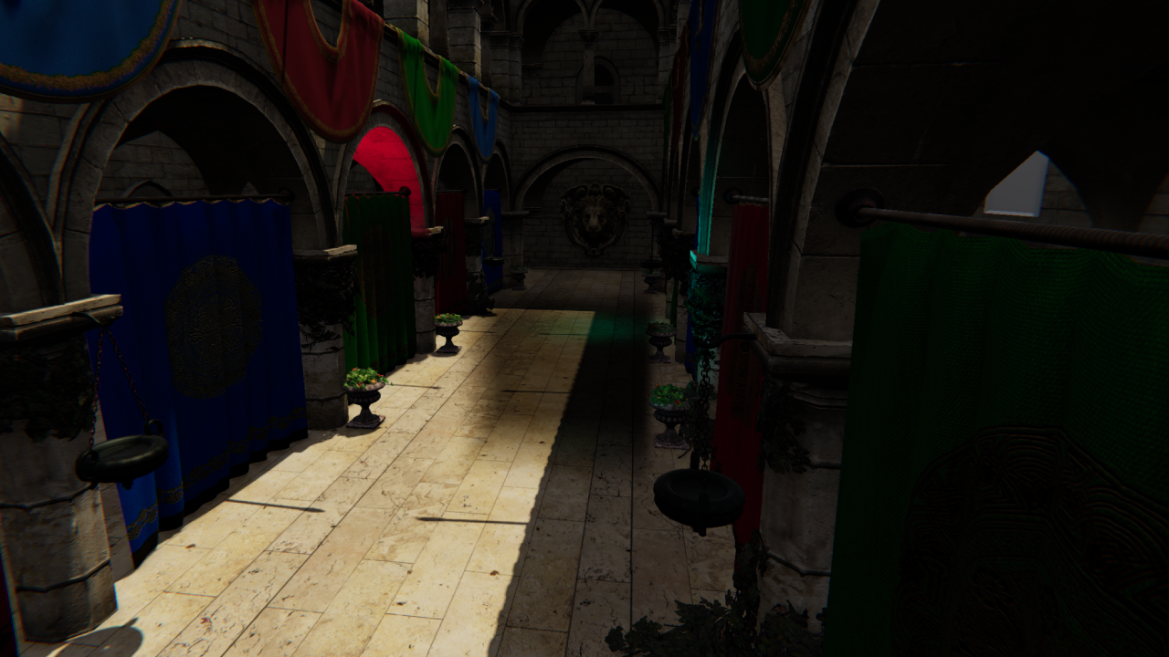
The following steps build up the final lighting contribution. This base image, with no fog applied, serves as the reference:
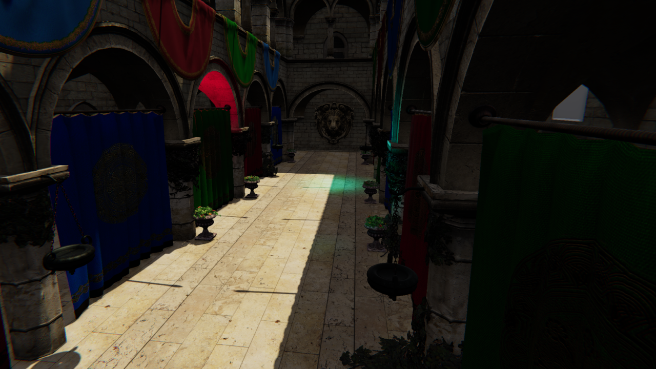
For each froxel, its world position is reconstructed, then three light types are evaluated and combined with the scattering coefficient and emissive into a source term:
float3 Lin = LinLocal + LinSun + LinIndirect;
float3 source = sigmaS * Lin + sigmaE;
Directional Light
The directional light is evaluated using cascaded shadow maps and the Henyey-Greenstein phase function:
float shadow = SampleCascadedShadow(float4(worldPos, 1));
float3 L = -normalize(DirectionalLightTransform._m02_m12_m22);
float phase = PhaseHG(dot(-L, L), phaseG);
return shadow * DirectionalLightColor.rgb * phase;
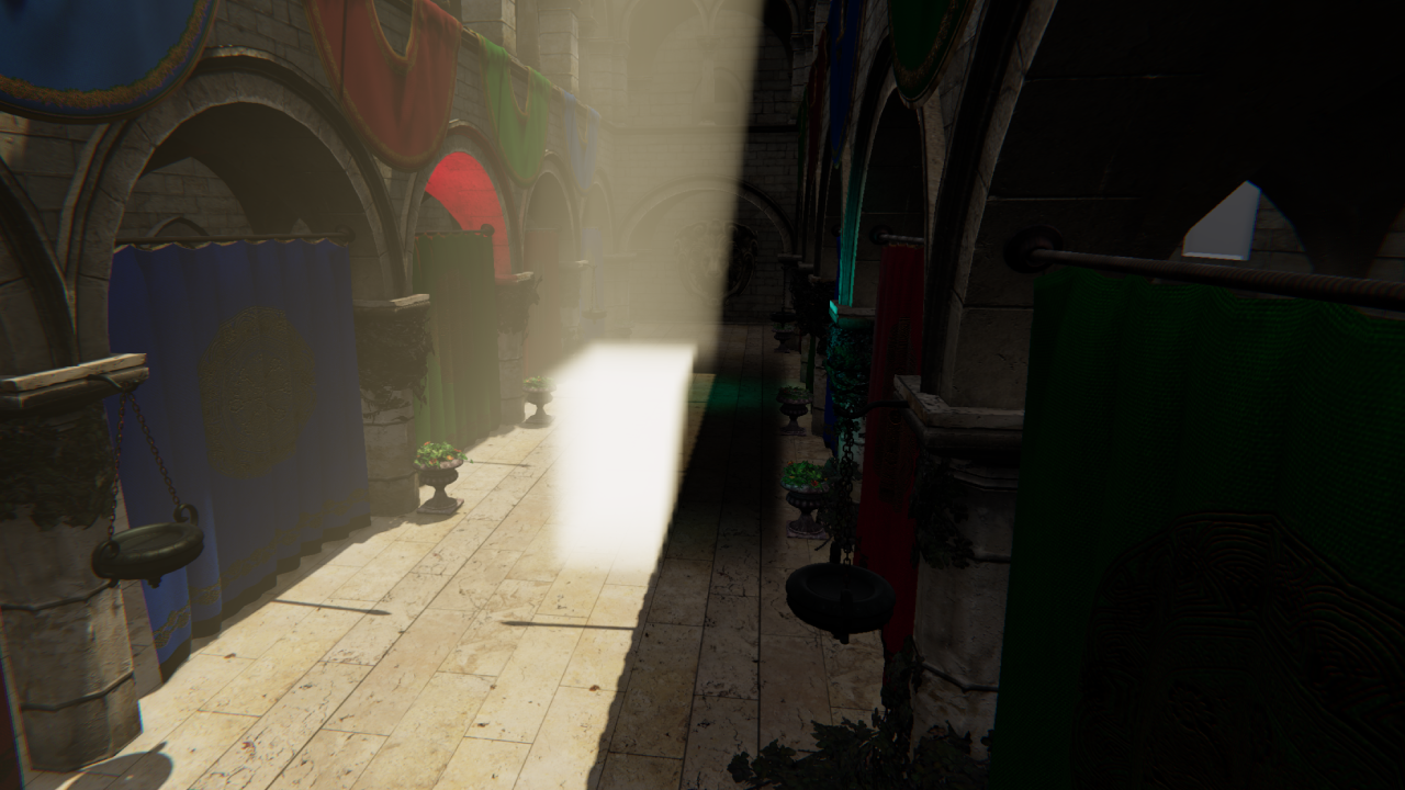
The darker regions inside the local volume are the transmittance term \(T_r\) at work — froxels deep inside the volume have had more light absorbed along the way, so less reaches the camera. As covered earlier, \(T_r \approx e^{-\sigma_t \cdot d}\) means the effect compounds with distance, which is why the shadowing looks volumetric rather than a flat darkening.
Local Lights
Local lights are managed using a clustered lighting structure — each froxel maps to a cluster tile and only evaluates the lights assigned to it, keeping cost manageable even with many lights in the scene. I built clustered lighting as part of this project, following this implementation guide.
if ((light.type & AffectsFog) == 0) continue;

float attenuation = GetLocalLightAttenuation(light, worldPos);
float phase = PhaseHG(dot(-L, L), phaseG);
float shadow = 1.f;
result += light.color * attenuation * phase * shadow;
A per-light flag lets artists opt individual lights out of fog contribution entirely. Local lights are evaluated without shadow maps — the engine doesn’t support per-light shadows, so lights bleed through geometry into the fog. Adding shadow support would be straightforward given the existing infrastructure.
Indirect Light
Indirect light is a flat ambient term. A more physically accurate approach would sample irradiance probes at the froxel world position — straightforward to add given the probe infrastructure, but out of scope for this project.
float3 EvaluateIndirectLight()
{
    return AmbientLightColor.rgb;
}
Pass 3 — Ray Marching
The final pass solves the in-scattering integral from the theory section. A single compute thread walks front-to-back through each XY column’s Z slices, analytically accumulating scattered light and transmittance.
The key is the closed-form solution from the theory section. Assuming constant scattering and extinction within a froxel, the integral over a slab of thickness \(D\) reduces to:
float stepLen = FroxelStepLength(texDepth, volumeDepth);
float Tr      = exp(-sigmaT * stepLen);
float3 Sint   = S * (1.0 - Tr) / sigmaT;

accum.rgb += Sint * accum.a;
accum.a   *= Tr;
accum.rgb accumulates total in-scattered light; accum.a tracks remaining transmittance. Each froxel’s contribution is already dimmed by everything in front of it via accum.a. The step length isn’t constant — it grows with depth because of the exponential slice distribution, so near slices contribute less depth than far ones:
float FroxelStepLength(uint texDepth, float volumeDepth)
{
    float z0 = ViewZFromSlice(texDepth,     volumeDepth);
    float z1 = ViewZFromSlice(texDepth + 1, volumeDepth);
    return z1 - z0;
}
The result per-froxel is written to FinalScatteringTransmittanceVolume (rgb = accumulated light, a = transmittance). The composite step in the pixel shader is then a single multiply-add — exactly the two-term structure of the volumetric rendering equation:
float4 fog    = FinalScatteringTransmittanceVolume.SampleLevel(sampler, float3(screenUV, slice), 0);
float3 result = sceneColor * fog.a + fog.rgb;
Temporal Integration
A problem you will inevitably run into is seeing individual froxel slices — the discrete depth boundaries of the froxel grid show up as visible banding in the fog volume.

Temporal integration is how we combat this: by jittering the sample position along the depth of each froxel and reprojecting against a history buffer, the slice boundaries wash out over successive frames.
This isn’t a separate pass — the jitter is applied during voxelization and lighting when reconstructing each froxel’s world position, and the reprojection, blend, and history write all happen at the end of the lighting shader.
Temporal is one of those areas where you can work forever — ghosting, disocclusion, flickering under fast motion, there is always another edge case to chase. What’s here solves the slicing problem well, but there is a lot of headroom to build on.
Jitter
Jittering the sample position along Z each frame ensures no two consecutive frames sample at the same depth within a froxel. Blended with history, this is what dissolves the visible slice boundaries:
float jitterZ = GetIGNJitter(); // IGN value in [0, 1), cycled by frame index
float3 jitteredWorldPos = GetJitteredFroxelWorldPosition(uv, slice, numSlices, jitterZ, ...);
Reprojection
To blend the current frame with the previous one, each froxel reprojects its world position into last frame’s clip space and samples the history buffer:
float4 prevClip  = mul(PrevViewProj, float4(worldPos, 1.0f));
float3 prevNDC   = prevClip.xyz / prevClip.w;
float2 prevUV    = float2(prevNDC.x * 0.5 + 0.5, -prevNDC.y * 0.5 + 0.5);
uint   prevSlice = SliceFromViewZ(FroxelCountZ, prevViewPos.z);
float3 prevUVW   = float3(prevUV, (prevSlice + 0.5) / FroxelCountZ);
float4 history = ScatteringExtinctionReadHistory.SampleLevel(LinearClampSampler, prevUVW, 0);
float4 result = lerp(currentValue, history, 0.95f);
The slice is reprojected alongside the UV — if the camera has moved, the same world position may now map to a different Z slice. The history is then blended with the current frame, with the weight reduced under fast motion to prevent smearing.
Going Further
There is a lot left on the table here. Some directions worth exploring:
- Velocity-based blend weight — derive the blend factor from the length of the reprojection delta rather than a fixed value, giving more aggressive rejection when the camera moves fast
- Neighborhood clamping — clamp the history sample to the min/max of the current froxel’s neighbors before blending, the standard TAA trick applied to the volume to reduce ghosting behind fast-moving objects
- Disocclusion detection — detect when a froxel has become newly visible (e.g. by comparing reprojected depth against the current froxel depth) and reset history weight to zero for that froxel
Reflection & Improvements
This was one of the most rewarding projects I’ve worked on — volumetric fog is one of those features where the visual payoff is immediate and obvious, and the underlying theory is deep enough to keep pulling you further in.
Beyond the fog itself, I learned a lot across the board. Working in DX11 at this level — managing structured buffers, UAVs, ping-pong resources, and multi-pass compute pipelines — gave me a much stronger mental model of how the GPU actually executes work. Building the clustered lighting acceleration structure alongside the fog was its own education: spatial data structures, tile binning, and keeping per-froxel cost bounded. And diving into participating media theory through PBRT gave me a new appreciation for how much physically-based rendering there is left to explore.
A few things I’d want to add or improve going forward:
Fog fallback — as noted earlier, pushing FogFarPlane too far causes the distant slices to become extremely wide, visibly degrading quality. The proper solution is a cheap analytic fog fallback that kicks in beyond the froxel grid’s range Most engines do exactly this, treating the froxel volume as a high-quality near-field solution and falling back to a cheaper approximation for everything beyond it.
3D density textures — sampling a scrolling 3D noise texture during voxelization would allow the fog density to vary spatially in interesting ways. Animating the UV offset over time would simulate wind moving through the volume, something that’s very hard to achieve convincingly with analytic volumes alone.
Local light shadows — local lights currently bleed through geometry into the fog. The fix is per-light shadow maps sampled during the lighting pass, but generating and managing those for an arbitrary number of lights is a non-trivial system to build correctly.
Better temporal integration — reprojection and blending can always be improved. Disocclusion handling, better neighbourhood clamping strategies, and more robust motion weighting are all areas with room to grow. As mentioned earlier, this is something that can always be improved and is something I plan to keep working on.
Global illumination — the indirect light term is currently a flat ambient constant. Sampling irradiance probes at each froxel’s world position would give spatially varying indirect light that responds to the scene, making the fog feel much more grounded in its environment.
Particle integration — the most complex addition would be voxelizing the particle system into the froxel grid during the voxelization pass. Particles can already carry density and scattering information; the challenge is projecting them into the correct froxels efficiently and without aliasing. Done well, this would allow smoke, sparks, and other effects to interact correctly with the volumetric lighting.
Who knows — 3D density textures and particle integration might be something I have time to add during our 7th and last game project at The Game Assembly.
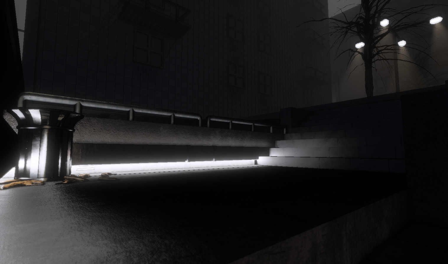
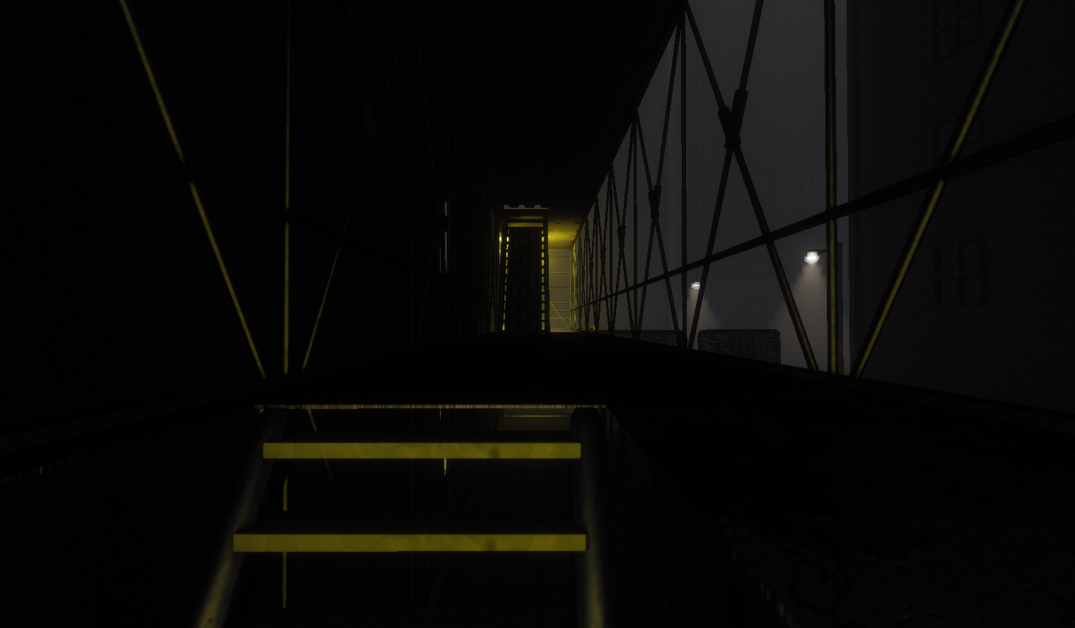
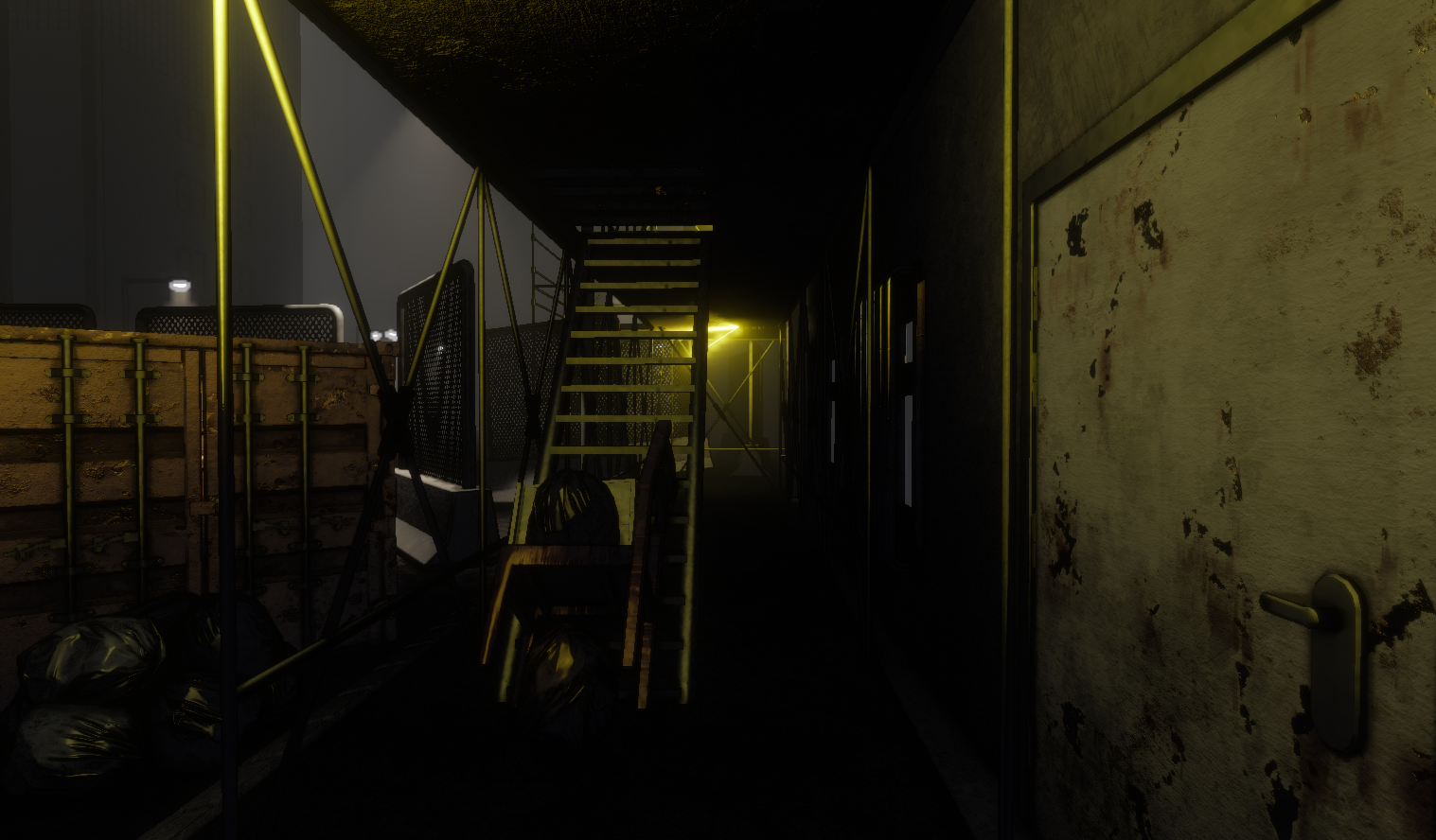
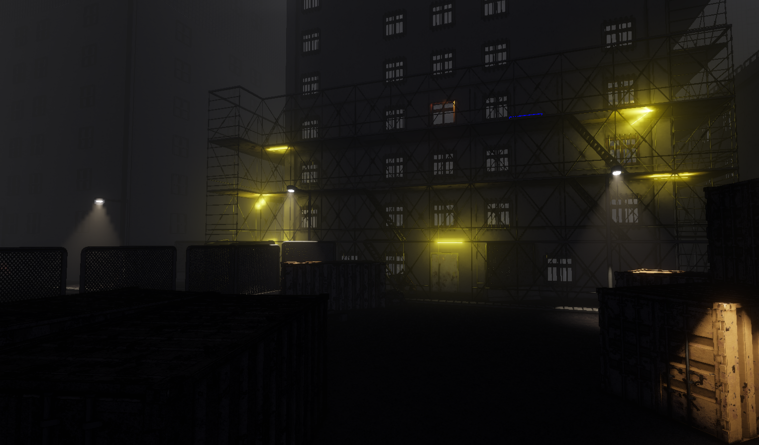
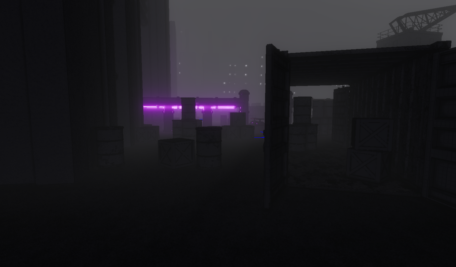
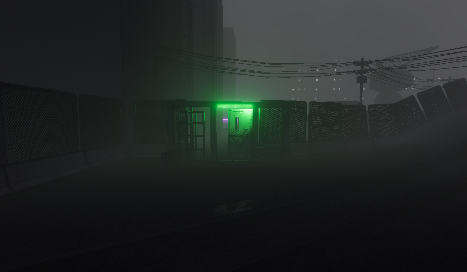
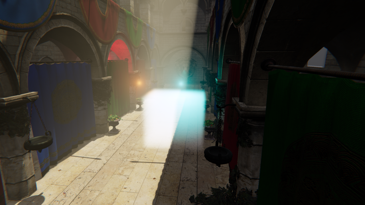
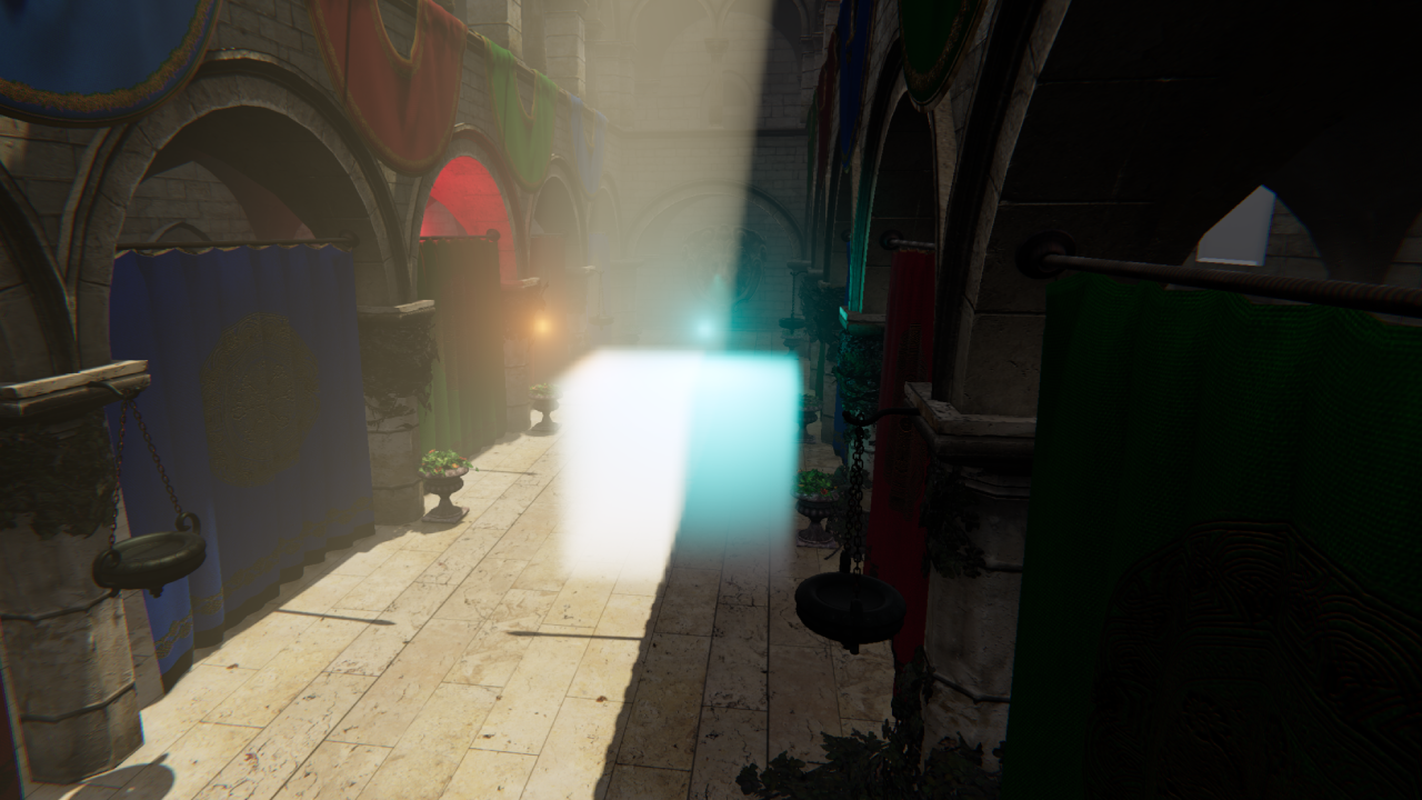
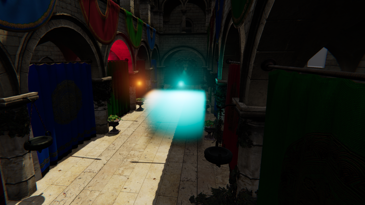
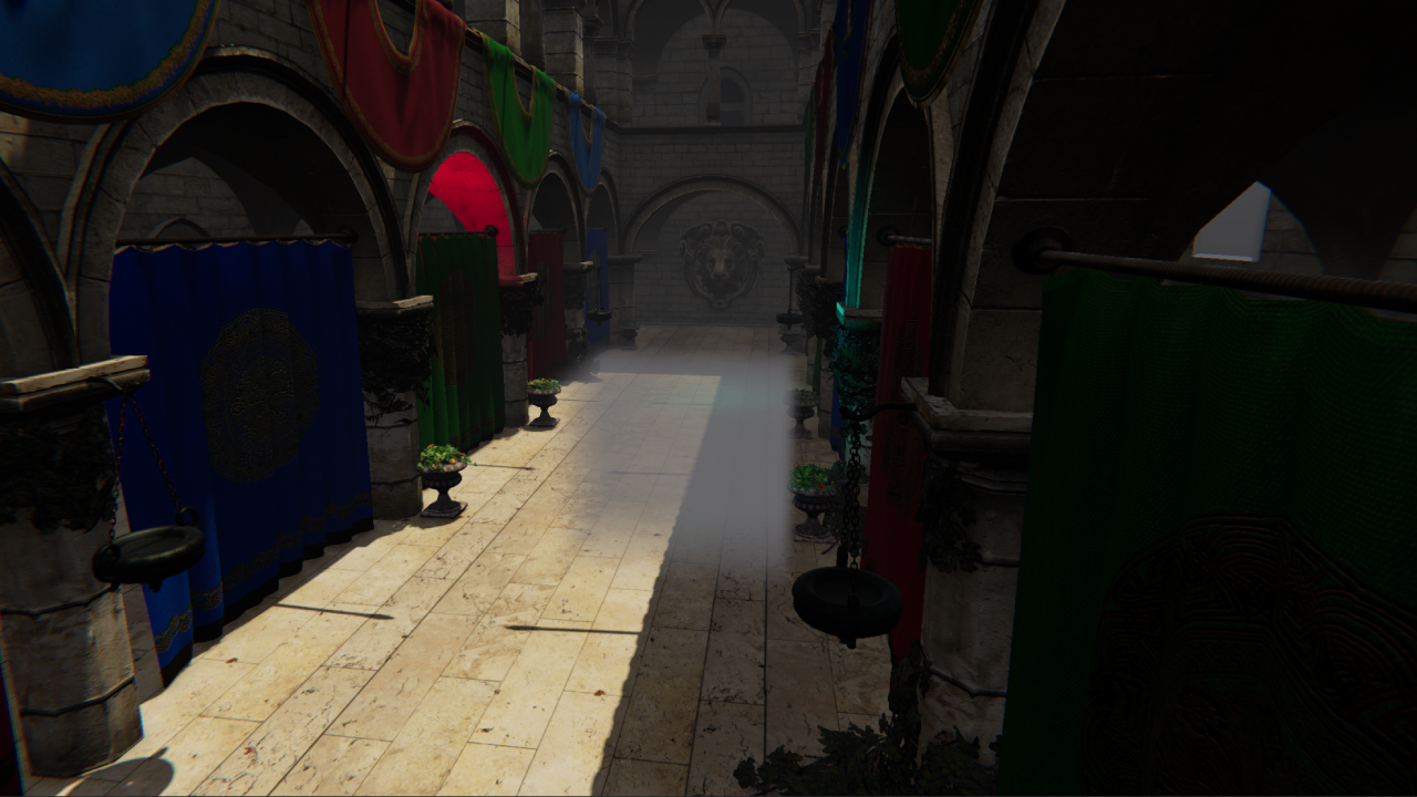
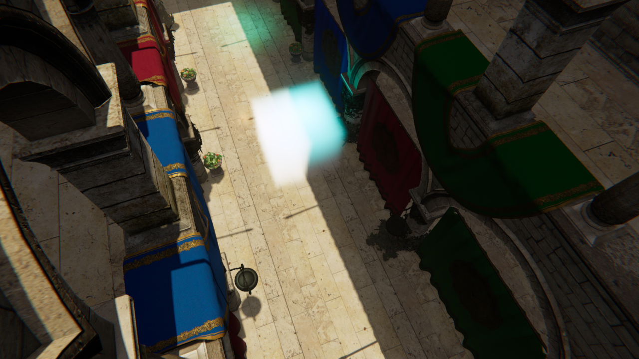
Screenshots
These are work in progress screenshots from our 6th game project at The Game Assembly. The game has a noir aesthetic where only surfaces directly affected by light receive color — everything else falls into desaturated shadow. The volumetric fog slots naturally into this: it picks up colored light and carries it into the environment, adding mood and atmosphere that the surface-only lighting can’t provide on its own.